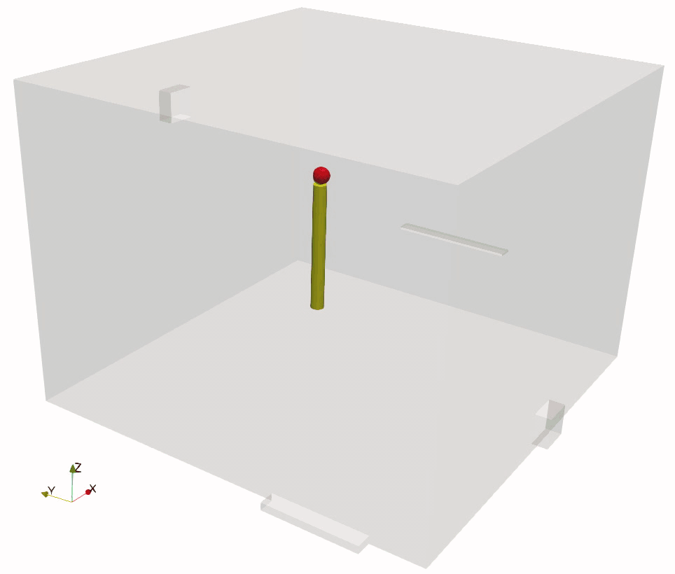
The object-oriented Python library developed in-lab was used to simulate the particles in the animation above. While the lab has publications in scientific journals using this code, the library is still in development and remains unpublished so I will not be including any code on this page. The mathematical methods used in the library will be discussed here as well as a brief overview of the structure of the library.


The structure of the codebase is as follows:
1. An execution script that reads additional command line inputs to find the input file.
2. An object is created with properties from an input text file passed as a command line argument.
3. An object is created from the CFD data indicated in the input file and contains the grid spatial data and any relevant fields such as velocity, temperature, and pressure.
4. An object is created containing properties that will be written to the output files. The values of these properties are updated throughout the simulation.
5. An object is created that performs the computations related to the particle physics, updates the values in the object from step 4, writes the output file for the current timestep, and repeats for the entire simulation time specified in the input file.


I am not the sole developer of this codebase, but have made significant contributions to the existing computational classes and created new computational classes as required by my research. The animation at the top of this page was created using tracer particle dynamics which have the following governing equation:

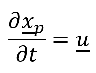
where x_p denotes the position of the particle and u denotes the fluid velocity at the particle’s position. In words, this equation says that the velocity of the particle (time derivative of position) exactly matches the velocity of the fluid at the same location. While this is never actually true, particles of a sufficiently small size can be approximated as tracers with minimal error. The computational class dictating this simulation was initially developed before I joined the lab, but I made significant alterations to the code to improve performance and add features.

Particles of this size, even in air, can experience random motion imposed by collision with other molecules. The addition of a stochastic term (W) in the tracer equation accounts for this random effect as follows:

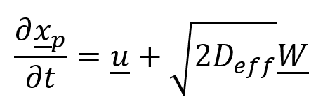
where D_eff scales the effect of this random motion and is specific to the system. Again, the computational class dictating this simulation was initially developed before I joined the lab, but I added important features such as adding random motion based on local turbulence effects. I will not include this governing equation because the lab does not have any publications with this feature yet.

For particles that are not of sufficiently small size, or where inertial effects are required by the focus of the study, they can be modeled with the following governing equation:

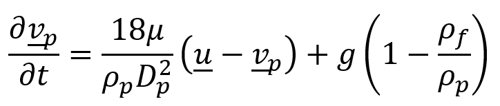
where the acceleration is now the particle property being integrated. The first term in this equation represents the effect on the particle due to differences in the particle and fluid velocity and is scaled by the fractional term out front. The inverse of this fractional term is referred to as the momentum response time and is the time it takes a particle released from rest to reach 63% of the freestream velocity. The second term in this equation is the combination of gravity and buoyancy effects on the particle.

Each of these three governing equations are present in the library. I was responsible for the creation of the code based on the third governing equation. I used the existing framework based on the first two governing equations but made significant improvements to the performance and creating output fields of relevant particle properties.