Background

The purpose of this script is to determine the losses of a solar array due to shading that occurs from the shadow of solar panels falling onto the next row. This calculation is necessary because if solar panels are placed far enough apart that their shadow does not fall onto other panels then the capacity factor of the array will decrease because most of the sunlight will not hit any panel. Optimization of the solar array must be conducted in order to determine the ideal distance between rows and panels that minimizes the shading losses and maximizes the energy captured.

Assumptions

This model assumes that there is no change in elevation between the panels. It also assumes that there is no shading from surrounding structures, e.g. environmental shading.

Inputs

Section 1 contains user defined physical attributes of the solar array system. Section 2 will import a 2D matrix representing the solar panel array, the direct normal irradiance at the location, and the Sky Diffusivity for each month.

Section 1: System Values

Below are values that are inherent to the system based, on the physical location and the system attributes.

This includes the height and width of the panels, the tilt relative to the ground, the azimuth of the system, how much space is between each panel, and how much space is between each row. All length values are in cm.

An array is then created that represents the surface of a single panel and the space between it and the next panel in that row.

L represents the distance between a spot on one panel and the corresponding location on the next panel. This is necessary to calculate due to how row spacing is defined for solar array systems, as the horizontal distance between the top of one panel to the bottom of the corresponding panel in the next row.

import numpy as np
latitude = 32.39
lat_rad = latitude*np.pi/180
longitude = -106.74
standard_long = -105
beta = 32.39
tilt = beta * np.pi/180
panel_azimuth = (-10)*np.pi/180
rho = 0.2
H, W = int(146), int(202)
panel_spacing = int(0 * 2.54)
row_spacing = 35 * 2.54
panel_dims = np.concatenate((np.ones((H,W)),np.zeros((H,panel_spacing))),axis=1).astype(bool)
L = row_spacing + H*np.cos(tilt)

Section 2: Evaluation Data

This section imports Direct Normal Irradiance and Sky Diffusivity (which is assumed to be constant for each month). DNI should be a column for each time point being evaluated and Sky Diffusivity should be a list of 12 values.

If multiple years are being evaluated, the DNI data for each year must be put in a different column because they will be averaged in this section if this is the case.

dni = np.loadtxt('DNI.txt')
sky_diffusivity = np.loadtxt('sky_diffusivity.txt')
if dni.ndim != 1:
    dni = np.average(dni,axis=1)

Section 3: Array Creation

Based on the timescale of the DNI imported, this will set up some of the arrays needed to calculate total insolation.

numDays = 365
days_in_month = np.array([31, 28, 31, 30, 31, 30, 31, 31, 30, 31, 30, 31])
julian_date = np.linspace(1,numDays,numDays)
numHours = 24*numDays
hours = np.linspace(0,numHours-1,numHours)
time_resolution = int(len(dni) / numHours)
julian_date_array = np.repeat(julian_date,24*time_resolution)
if time_resolution != 1:
    hours = np.repeat(hours,time_resolution)
    minutes_array = np.linspace(0,60,time_resolution+1)
    minutes_array = np.tile(minutes_array[minutes_array != 60],numHours)

Section 4: Calculations

This section performs calculations on the Direction Normal Irradiance and global position to get the insolation, solar altitude, and solar azimuth for each time point being evaluated.

The computational time to compute the shading is significant. To reduce this time, the entries of the calculated data where the insolation is 0 or negative are removed since no solar power is produced at these times.

declination_angle = 23.45*np.sin((360/365)*(284+julian_date_array))*np.pi/180
B = (360/364)*(julian_date_array-81)*np.pi/180
et = 9.87*np.sin(2*B) - 7.53*np.cos(B)-1.5*np.sin(B)
solar_time = (60*hours)+minutes_array+et+(4*(standard_long-longitude))
h_s = ((solar_time-720)/4)*np.pi/180
solar_altitude = np.arcsin(np.sin(lat_rad)*np.sin(declination_angle)+np.cos(lat_rad)*np.cos(declination_angle)*np.cos(h_s))
solar_azimuth = np.arcsin(np.cos(declination_angle)*np.sin(h_s)/np.cos(solar_altitude))
incident_angle = np.cos(solar_altitude)*np.cos(solar_azimuth-panel_azimuth)*np.sin(tilt)+np.sin(solar_altitude)*np.cos(tilt)
C_array = np.repeat(np.repeat(sky_diffusivity,days_in_month),24*time_resolution)
I_bc = dni*incident_angle
I_dc = np.multiply(C_array,dni)*(1+np.cos(tilt)/2)
I_rc = rho*dni*(np.sin(solar_altitude)+C_array)*(np.sin(0.5*tilt)**2)
insolation = I_bc+I_dc+I_rc
solar_altitude = solar_altitude[insolation>0]
solar_azimuth  = solar_azimuth[insolation>0]
insolation = insolation[insolation>0]
rel_solar_azimuth  = (solar_azimuth - panel_azimuth)
tot_insolation = sum(insolation)
numTimes = len(insolation)

Section 5: The Solar Array

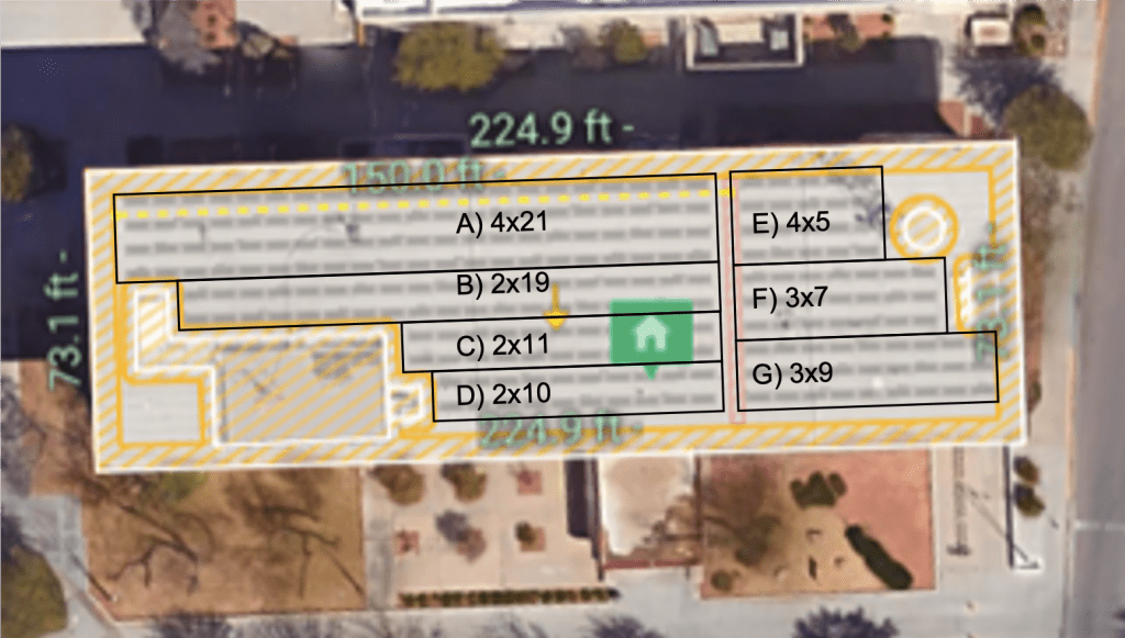
Define entire solar array as a single matrix, with 0 in spaces without panel and 1 in spaces with panel.

Row ordering starts with front row with respect to the sun, and the column ordering goes West to East. In other words, the matrix is flipped vertically compared to the physical solar array.

An example of what this matrix looks like would be:

0, 0, 0, 0, 0, 0, 0, 0, 0, 0, 0, 1, 1, 1, 1, 1, 1, 1, 1, 1, 1, 0, 1, 1, 1, 1, 1, 1, 1, 1, 1

0, 0, 0, 0, 0, 0, 0, 0, 0, 0, 0, 1, 1, 1, 1, 1, 1, 1, 1, 1, 1, 0, 1, 1, 1, 1, 1, 1, 1, 1, 1

0, 0, 0, 0, 0, 0, 0, 0, 0, 0, 1, 1, 1, 1, 1, 1, 1, 1, 1, 1, 1, 0, 1, 1, 1, 1, 1, 1, 1, 1, 1

0, 0, 0, 0, 0, 0, 0, 0, 0, 0, 1, 1, 1, 1, 1, 1, 1, 1, 1, 1, 1, 0, 1, 1, 1, 1, 1, 1, 1, 0, 0

0, 0, 1, 1, 1, 1, 1, 1, 1, 1, 1, 1, 1, 1, 1, 1, 1, 1, 1, 1, 1, 0, 1, 1, 1, 1, 1, 1, 1, 0, 0

0, 0, 1, 1, 1, 1, 1, 1, 1, 1, 1, 1, 1, 1, 1, 1, 1, 1, 1, 1, 1, 0, 1, 1, 1, 1, 1, 1, 1, 0, 0

1, 1, 1, 1, 1, 1, 1, 1, 1, 1, 1, 1, 1, 1, 1, 1, 1, 1, 1, 1, 1, 0, 1, 1, 1, 1, 1, 0, 0, 0, 0

1, 1, 1, 1, 1, 1, 1, 1, 1, 1, 1, 1, 1, 1, 1, 1, 1, 1, 1, 1, 1, 0, 1, 1, 1, 1, 1, 0, 0, 0, 0

1, 1, 1, 1, 1, 1, 1, 1, 1, 1, 1, 1, 1, 1, 1, 1, 1, 1, 1, 1, 1, 0, 1, 1, 1, 1, 1, 0, 0, 0, 0

1, 1, 1, 1, 1, 1, 1, 1, 1, 1, 1, 1, 1, 1, 1, 1, 1, 1, 1, 1, 1, 0, 1, 1, 1, 1, 1, 0, 0, 0, 0

Which corresponds to the following example solar array:

solar_array = np.loadtxt('thomasAndBrown.txt', delimiter=',', dtype=bool)
[z, c] = solar_array.shape

Section 6: 3D Matrix Representing the System

This section creates a 3D matrix representation of the solar array system to a 1 square cm resolution.

The number of columns in this matrix will be such that it represents the actual width of the array system to the nearest centimeter.

The total area is also calculated for later purposes.

cols = int(c * (W+panel_spacing))
solar_sys_mat_3D = np.zeros((H,cols,z))
for i in range(z):
    row_vals = panel_dims*solar_array[i,1]
    for j in range(1,c):
         new_entry = panel_dims * solar_array[i,j]
         row_vals = np.concatenate((row_vals,new_entry),axis=1)
    solar_sys_mat_3D[:, :, i] = row_vals
solar_sys_mat_3D = solar_sys_mat_3D.astype(bool)
total_area = sum(sum(sum(solar_sys_mat_3D)))

Section 7: Vertical Shading Displacement

This sections calculates the height of the shadow on the row behind it. This calculation is complicated geometrically so I have a diagram here and an explanation of the diagram below.

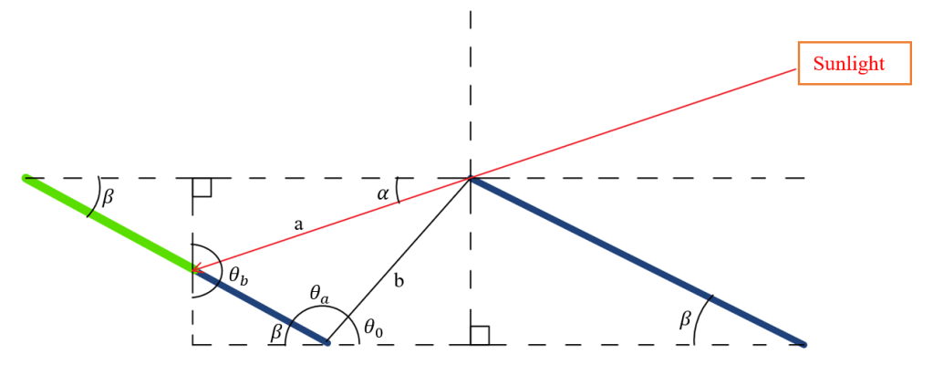
The goal of this section is to find the length of the green segment, then subtract that from the height of a panel which gives the index of the highest point that is shaded on the panel. Now let’s go through the geometry.

θ0 is the inverse tangent of the opposite and adjacent sides, both of which are determined by the physical values of the system, so this angle does not change during the evaluation.

θa can be found by subtracting β and θ0 from 180°. Since this angle is also based on the physical values of the system, this angle does not change.

θb can be found by subtracting the adjacent angles from 180°. These adjacent angles are each part of right triangles and can be found by the evaluation of 90°-α and 90°-β. Simplifying the resulting equation shows that θa=α+β. This value also will change in the evaluation based on the angle α.

The line indicated by the letter ‘b’ can be found from the square root of the sum of the squares of the other two sides in the right triangle. The other sides are the row spacing and sin(β) which are again system values which do not change.

The line indicated by the letter ‘a’ represents the distancβe from the top of the first solar panel, to the point it hits on the next panel. This distance will change throughout the evaluation and based on the values found earlier, can now be found using the Law of Sines a/sin(θa)=b/sin(θb).

Now that we have ‘a’, we can find the section of length that we set out to find, which comes from the realization that the vertical line segment above the green line is shared by two right triangles, which yields the expression asin(α)=length(sin(β)).

Subtracting this length from the height of the panel gives us the index of the highest point on the panel that is shaded.

theta_0 = np.arctan2(H*np.sin(tilt), row_spacing)
theta_a = (180-(theta_0*180/np.pi)-beta)*np.pi/180
theta_b = (solar_altitude+tilt)
b = np.sqrt(row_spacing**2+H**2*np.sin(tilt)**2)
a = b*np.sin(theta_a)/np.sin(theta_b)
shading_vert_disp = a * np.sin(solar_altitude)/np.sin(tilt)
ind = (H-shading_vert_disp).astype(int)

Section 8: Horizontal Shading Displacement

This section calculates the horizontal displacement of the shadow from one panel onto the row behind it. A diagram of this calculation is as follows:

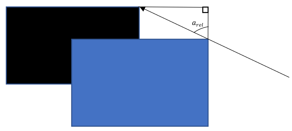
Where the actual displacement is found by L*tan(arel), where L is the distance between corresponding points calculated earlier and arel is the relative azimuth.

The shading condition calculated here indicates the direction that a panel’s shadow falls, i.e. if the shading condition is negative then the sun’s azimuth is to the East of the panel azimuth and the panel’s shadow is to the West.

shading_horiz_disp = (abs(np.multiply(L,np.tan(rel_solar_azimuth)))).astype(int)
shading_condition = np.sin(rel_solar_azimuth*np.pi/180)

Section 9: Shading Loss Calculation

Shading is intialized as a matrix of boolean Trues with one less sheet than the 3D system matrix because the last row will not cast a shadow on any other panels. The calculated_insolation value is initialized as 0 and is a running sum for each loop iteration. The no_shading_condition is the total area of the panels that are not in the front row. The front row area value is included in the insolation calculation and is separate because this row does not experience shading based on the assumptions of this model.

The first if-else statement in the loop checks if the top of the shadow falls on the panel, or above the panel. If the shadow does not fall on the panel then there is no shading on the panels and the shading calculation does not need to be completed, which sets to unshaded area to the no_shading_area condition. If the shadow is at or above the top of the next panel, then the only displacement necessary to incorporate is the horizonatal shading.

The nested if-else statements determine the direction that the shadow moves horizontally and then assigns the shading to the correct indices based on the displacements calculated.

The shadow is calculated as the inverse of the corresponding area of all rows but the last one. By using the inverse of these elements, in an index where a panel was there will now be a False because there is shade in this location, and where there is no panel there will now be a True at this location.

Now that the shading has been calculated it is multiplied element by element with all sheets of the system matrix except for the first row, and the result is summed to get the total unshaded area.

Now that the shading has been calculated, the unshaded area is added to the front row area to get the total area that receives sunlight, then divided by the total area, and multiplied by the insolation at this time to get the actual energy produced by the solar system array. The shading matrix is then reset to all True values for the next iteration.

The loss that the system experiences due to shading is one minus the fraction of the calculated energy production to the theoretical energy production if the system experienced no shading.

shading = np.ones((H,cols,z-1)).astype(bool)
calculated_insolation = 0
no_shading_area = sum(sum(sum(solar_sys_mat_3D[:,:,1:z])))
front_row_area = sum(sum(solar_sys_mat_3D[:,:,0]))
indicators = np.linspace(0.1*numTimes,numTimes,10).astype(int)
j = 0
print('Calculating shading loss. This will take a few minutes, please wait...')
for ii in range(numTimes):
 if ind[ii] > 0 and ind[ii] < H:
     if shading_condition[ii]  0:
         shading[0:ind[ii],shading_horiz_disp[ii]:cols,:]=np.invert(solar_sys_mat_3D[H-ind[ii]:H,shading_horiz_disp[ii]:cols,0:z-1])
     else:
         shading[0:ind[ii], :, :] = np.invert(solar_sys_mat_3D[H-ind[ii]:H,:,0:z-1])
     unshaded_area = sum(sum(sum(np.multiply(solar_sys_mat_3D[:,:,1:z], shading))))
  elif ind[ii] >= H:
     if shading_condition[ii]  0:
         shading[:,shading_horiz_disp[ii]:cols,:]=np.invert(solar_sys_mat_3D[:,shading_horiz_disp[ii]:cols,0:z-1])
     else:
         shading[:,:,:] = np.invert(solar_sys_mat_3D[:,:,0:z-1])
     unshaded_area = sum(sum(sum(np.multiply(solar_sys_mat_3D[:,:,1:z], shading))))
  else:
     unshaded_area = no_shading_area
  calculated_insolation = calculated_insolation + ((unshaded_area+front_row_area)/total_area)*insolation[ii]
  shading[:,:,:] = True
  if ii+1 == indicators[j]:
     print('...',10*(j+1),'% complete ...')
     j += 1shading_loss = 1 - (calculated_insolation / tot_insolation)print('')
print('Shading loss = ', round(shading_loss*100,2), '%')